【AI程设】scikit-learn 基础
AI程设课上教的 scikit-learn
内容来源于 北京交通大学 计算机学院 人工智能专业 大二专业课 人工智能程序设计
scikit-learn 处理数据
读取自带数据集
1
2
3
4
5
6
7
8
9
10
11
from sklearn.datasets import load_breast_cancer

cancer = load_breast_cancer()

cancer_data = cancer['data'] ## 取出数据集的数据

cancer_target = cancer['target'] ## 取出数据集的标签

cancer_names = cancer['feature_names'] ## 取出数据集的特征名

cancer_desc = cancer['DESCR'] ## 取出数据集的描述信息
数据集划分
划分函数:
train_test_split()直接传入数据与标签
test_size = ...train_size = ...二选一传入小数random_state = ...传入随机种子,默认42shuffle = boolean代表是否进行有放回抽样stratify = ...接受array或None,用传入的标签进行分层抽样
1
2
3
4
5
6
from sklearn.model_selection import train_test_split

data_train, data_test, target_train, target_test = train_test_split(cancer_data, cancer_target,
                                                                    test_size=0.2,
                                                                    random_state=42,
                                                                    stratify=cancer_target)
数据预处理与降维
from sklearn.preprocessing import ...离差标准化:
MinMaxScaler, 标准差标准化:StandardScaler, 归一化:Normalizer二值化处理:
Binarizer, 独热编码处理:OneHotEncoder, 自定义函数变换:FunctionTransformer需要先用
.fit()针对训练集生成规则再用
.transform()对数据集进行处理
1
2
3
4
5
6
7
from sklearn.preprocessing import MinMaxScaler, StandardScaler, Normalizer, Binarizer, OneHotEncoder, FunctionTransformer

Scaler = MinMaxScaler().fit(cancer_data_train) # 生成规则
# 将规则应用于训练集
cancer_trainScaler = Scaler.transform(cancer_data_train)
# 将规则应用于测试集
cancer_testScaler = Scaler.transform(cancer_data_test)
PCA 降维
需要根据数据本身特征数量决定是否进行降维,如果本来特征数量就很少(比如小于 10 个),就没有降维的必要
from sklearn.decomposition import PCAn_components = ...降维后的数据是几维。未指定时,所有特征都会被保留下来需要先用
.fit()针对训练集生成规则再用
.transform()对数据集进行处理
1
2
3
4
from sklearn.decomposition import PCA
pca_model = PCA(n_components = 10).fit(cancer_trainScaler) ##生成规则
cancer_trainPca = pca_model.transform(cancer_trainScaler) ##将规则应用于训练集
cancer_testPca = pca_model.transform(cancer_testScaler) ##将规则应用于测试集
构建分类模型 - 以 SVM 举例
构建模型
from sklearn.svm import SVC直接
.fit(data, target)即可
1
2
3
4
5
6
7
8
9
10
11
12
13
14
15
16
17
18
19
20
21
22
23
## 4. 建立SVM模型
svm = SVC().fit(cancer_trainStd, cancer_target_train)
print('建立的SVM模型为:\n', svm)

## 5. 预测训练集结果
cancer_target_pred = svm.predict(cancer_testStd)
print('预测前20个结果为:\n', cancer_target_pred[:20])

## 6. 求出预测和真实一样的数目
true = np.sum(cancer_target_pred == cancer_target_test)
print('预测对的结果数目为:', true)
print('预测错的的结果数目为:', cancer_target_test.shape[0] - true)
print('预测结果准确率为:', true / cancer_target_test.shape[0])

'''
建立的SVM模型为:
 SVC()
预测前20个结果为:
 [1 0 0 0 1 1 1 1 1 1 1 1 0 1 1 1 0 0 1 1]
预测对的结果数目为: 111
预测错的的结果数目为: 3
预测结果准确率为: 0.9736842105263158
'''
评价模型
from sklearn.metrics import ...(target_test, pred_test)accuracy_score()准确率precision_score()精确率recall_score()召回率f1_score()F1 值cohen_kappa_score()Kappa 系数分类模型评价报告:
classification_report()
1
2
3
4
5
6
7
8
9
10
11
12
13
14
15
16
17
18
19
20
21
22
23
24
25
26
from sklearn.metrics import accuracy_score, precision_score, recall_score, f1_score, cohen_kappa_score
accuracy_score(cancer_target_test, cancer_target_pred)
precision_score(cancer_target_test, cancer_target_pred)
recall_score(cancer_target_test, cancer_target_pred)
f1_score(cancer_target_test, cancer_target_pred)
cohen_kappa_score(cancer_target_test, cancer_target_pred)

from sklearn.metrics import classification_report
classification_report(cancer_target_test, cancer_target_pred)

'''
使用SVM预测breast_cancer数据的准确率为: 0.9736842105263158
使用SVM预测breast_cancer数据的精确率为: 0.9594594594594594
使用SVM预测breast_cancer数据的召回率为: 1.0
使用SVM预测breast_cancer数据的F1值为: 0.9793103448275862
使用SVM预测breast_cancer数据的Cohen’s Kappa系数为: 0.9432082364662903
使用SVM预测iris数据的分类报告为:
               precision    recall  f1-score   support

           0       1.00      0.93      0.96        43
           1       0.96      1.00      0.98        71

    accuracy                           0.97       114
   macro avg       0.98      0.97      0.97       114
weighted avg       0.97      0.97      0.97       114
'''
绘制 ROC 曲线
x, y, thresholds = roc_curve(target_test, pred_test)
1
2
3
4
5
6
7
8
9
10
11
from sklearn.metrics import roc_curve
import matplotlib.pyplot as plt
## 求出ROC曲线的x轴和y轴
fpr, tpr, thresholds = roc_curve(cancer_target_test, cancer_target_pred)
plt.figure(figsize = (10, 6))
plt.xlim(0, 1) ##设定x轴的范围
plt.ylim(0.0, 1.1) ## 设定y轴的范围
plt.xlabel('False Postive Rate')
plt.ylabel('True Postive Rate')
plt.plot(fpr, tpr, linewidth = 2, linestyle = "-", color = 'red')
plt.show()
构建聚类模型 - 以 Kmean 举例
Kmean 基础
from sklearn.cluster import KMeansKMeans(n_clusters = 3, random_state = 123)n_clusters = ...要聚几类.fit(data)进行数据拟合.predict(data)输入测试数据,输出聚类结果
1
2
kmeans = KMeans(n_clusters = 3, random_state = 123).fit(iris_dataScale) # 构建并训练模型
result = kmeans.predict([[1.5, 1.5, 1.5, 1.5]])
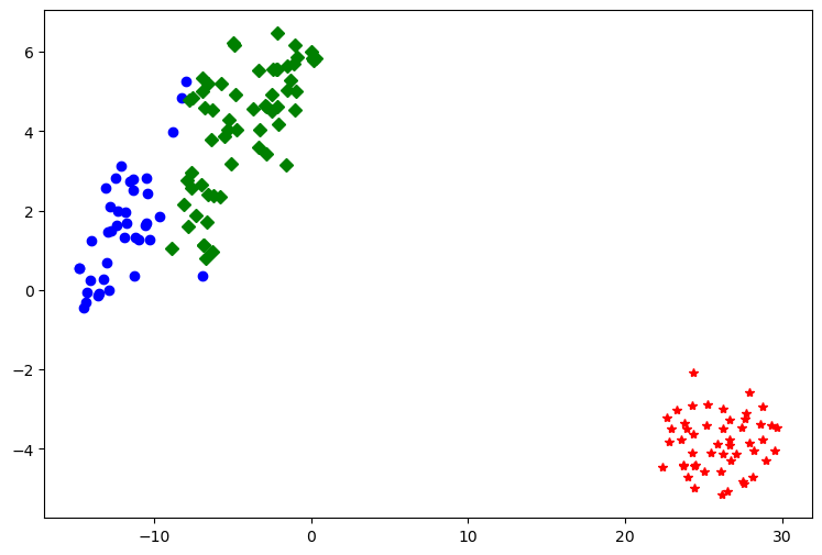
聚类结果可视化
TSNE函数降维后可视化from sklearn.manifold import TSNE
1
2
3
4
5
6
7
8
9
10
11
12
13
14
15
16
17
18
19
20
21
import pandas as pd
from sklearn.manifold import TSNE
import matplotlib.pyplot as plt

##使用TSNE进行数据降维,降成两维
tsne = TSNE(n_components=2,init='random', random_state=177).fit(iris_data)
##将原始数据转换为DataFrame
df = pd.DataFrame(tsne.embedding_) # embedding_

##将聚类结果存储进df数据表
df['labels'] = kmeans.labels_ ##提取不同标签的数据
df1 = df[df['labels'] == 0]
df2 = df[df['labels'] == 1]
df3 = df[df['labels'] == 2]

## 绘制图形
fig = plt.figure(figsize = (9, 6)) ##设定空白画布,并制定大小
##用不同的颜色表示不同数据
plt.plot(df1[0], df1[1], 'bo', df2[0], df2[1], 'r*', df3[0], df3[1], 'gD')
plt.savefig('聚类结果.png')
plt.show() ##显示图片
聚类结果评价
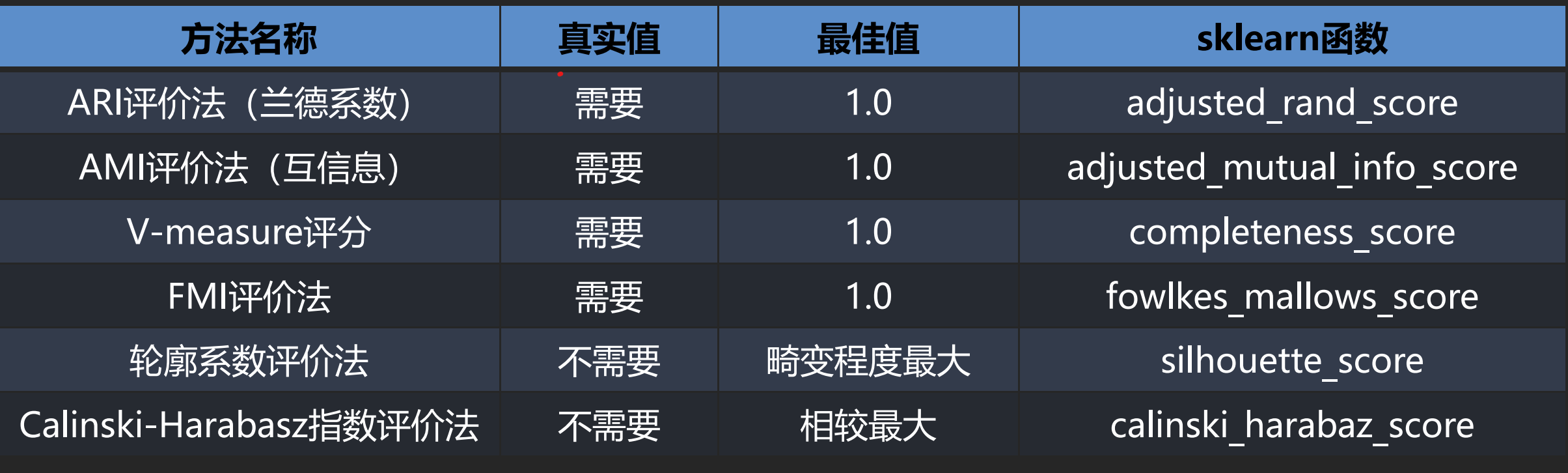
其中前4种方法均需要真实值的配合才能够评价聚类算法的优劣,后2种则不需要真实值的配合。
前四种:
(target, kmeans.labels_)后两种:
(data, kmeans.labels_)
构建回归模型 - 以 LinearRegression 为例
线性回归基础
from sklearn.linear_model import LinearRegression.fit(train_data, train_target)
1
2
3
clf = LinearRegression().fit(X_train,y_train)

y_pred = clf.predict(X_test)
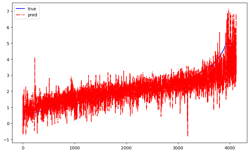
回归结果可视化
1
2
3
4
5
6
7
8
9
10
11
12
df = pd.DataFrame()
df["pred"] = y_pred
df["test"] = y_test
df.sort_values('test', axis = 0, ascending = True, inplace = True)

fig = plt.figure(figsize = (10, 6)) ##设定空白画布,并制定大小

plt.plot(range(y_test.shape[0]), df['test'], color = "blue", linewidth = 1.5, linestyle = "-")
plt.plot(range(y_test.shape[0]), df['pred'], color = "red", linewidth = 1.5, linestyle = "-.")
plt.legend(['true', 'pred'])
plt.savefig('xxxx')
plt.show() ##显示图片
回归结果评价
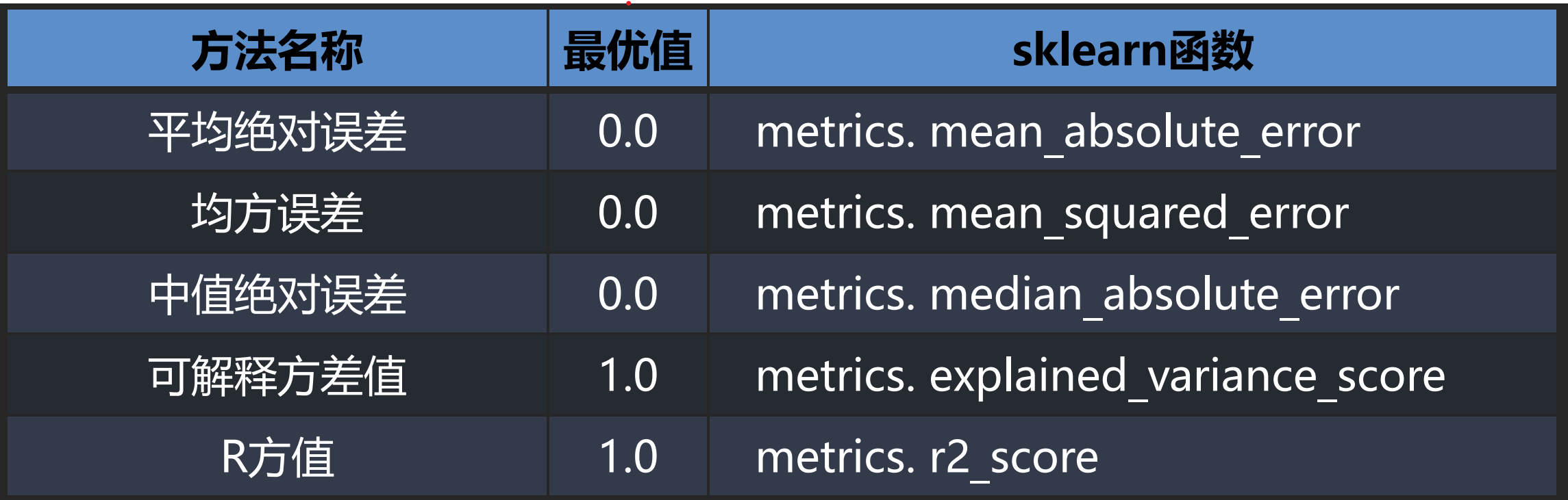
(target, y_pred)真实值 预测值