跟李沐动手学深度学习笔记第一部分 01-15

跟李沐动手学深度学习笔记

Posted Feb 17, 2025 Updated Feb 24, 2025

By ZhaiWangyuxuan

11 min read

01 - 03 忽略

04 数据操作 + 数据预处理

基本

  
import torch
x = torch.arange(12)

x.shape # 张量形状
# torch.Size([12])

x.numel() # 有多少元素
# 12

x = x.reshape(3, 4) # 改变形状

torch.zeros((2, 3, 4)) # 全零
torch.ones((2, 3, 4)) # 全一
torch.tensor([[1, 2, 3, 4], [5, 6, 7, 8]]) # 自定义

计算与连接

  
# 算术运算符被升级为按元素计算
x = torch.tensor([1.0, 2, 4, 8])
y = torch.tensor([2, 2, 2, 2])
x + y, x - y, x * y, x / y, x ** y  # **运算符是求幂运算

'''
(tensor([ 3.,  4.,  6., 10.]),
 tensor([-1.,  0.,  2.,  6.]),
 tensor([ 2.,  4.,  8., 16.]),
 tensor([0.5000, 1.0000, 2.0000, 4.0000]),
 tensor([ 1.,  4., 16., 64.]))
'''

# 更多计算
torch.exp(x)

# 把多个张量连接在一起
x = torch.arange(12, dtype=torch.float32).reshape(3, 4)
y = torch.tensor([[2.0, 1, 4, 3], [1, 2, 3, 4], [4, 3, 2, 1]])
torch.cat((x, y), dim=0), torch.cat((x, y), dim=1) # 按行连接 按列连接

'''
(tensor([[ 0.,  1.,  2.,  3.],
         [ 4.,  5.,  6.,  7.],
         [ 8.,  9., 10., 11.],
         [ 2.,  1.,  4.,  3.],
         [ 1.,  2.,  3.,  4.],
         [ 4.,  3.,  2.,  1.]]),
 tensor([[ 0.,  1.,  2.,  3.,  2.,  1.,  4.,  3.],
         [ 4.,  5.,  6.,  7.,  1.,  2.,  3.,  4.],
         [ 8.,  9., 10., 11.,  4.,  3.,  2.,  1.]]))
'''

x == y # 按元素判断

'''
tensor([[False,  True, False,  True],
        [False, False, False, False],
        [False, False, False, False]])
'''

x.sum()

# torch 也有广播机制
# 矩阵访问同 python [-1] [1:3]
# 可以同时为多个元素赋值相同的值

内存操作

  
# torch 也有广播机制
# 矩阵访问同 python [-1] [1:3]
# 可以同时为多个元素赋值相同的值

# 运行一些操作可能会导致为新结果分配内存
x = torch.arange(12).reshape(3, 4)
before = id(x) # 可以看作是 c++ 的指针

y = torch.ones((3, 4))
x = x + y
id(x) == before
# False

# 执行原地操作
z = torch.zeros_like(y) # 创建一个全 0 的形状同 y 的张量
print('id(z):', id(z))
z[:] = x + y
print('id(z):', id(z))
# z 的内存没有变化

before = id(x)
x += y
id(x) == before
# 在后续计算中不重复使用之前的结果，为了减少内存开销和计算开销

转换

  
# 转换为 NumPy 张量
A = x.numpy()
B = torch.tensor(A)
type(A), type(B)
# (numpy.ndarray, torch.Tensor)

# 将大小为 1 的张量转换为 Python 标量
a = torch.tensor([3.5])
a, a.item(), float(a), int(a) # item() 函数将张量转换为 Python 标量
# (tensor([3.5000]), 3.5, 3.5, 3)

数据预处理

  
import pandas as pd
data = pd.read_csv(file)

# 处理缺失数据
inputs, outputs = data.iloc[:, 0:1], data.iloc[:, 2]
inputs = inputs.fillna(inputs.mean()) # 填充缺失值
inputs = pd.concat((inputs, data.iloc[:, 1]), axis = 1) # 缺失的数值处理
inputs

# 处理类别值或离散值 可以将 NaN 视为一个类型
inputs = pd.get_dummies(inputs, dummy_na=True)

# 将 inputs 中的 T F 转换为 1 0
inputs = inputs * 1
inputs

'''
	NumRooms	Alley_Pave	Alley_nan
0	  3.0	        1	        0
1	  2.0	        0	        1
2	  4.0	        0	        1
3	  3.0	        0	        1
'''

# 此时 inputs 与 outputs 中的所有条目都是数值类型，可以转换为张量了
X, y = torch.tensor(inputs.values), torch.tensor(outputs.values)
X, y

# 一般类型都是 torch.float64
# 但是比较慢
# 普遍都用 torch.float32

'''
(tensor([[3., 1., 0.],
         [2., 0., 1.],
         [4., 0., 1.],
         [3., 0., 1.]], dtype=torch.float64),
 tensor([127500, 106000, 178100, 140000]))
'''

特别注意尽量不要改东西

  
# 尽量别去改东西
a = torch.arange(12)
b = a.reshape((3, 4))
b[:] = 2
a # 显然这里把 a 也给改了, 但我们明明只改了 b

'''
tensor([2, 2, 2, 2, 2, 2, 2, 2, 2, 2, 2, 2])
'''

torch 的 tensor 与 numpy 的 array 不相似

05 线性代数

Frobenius 范数

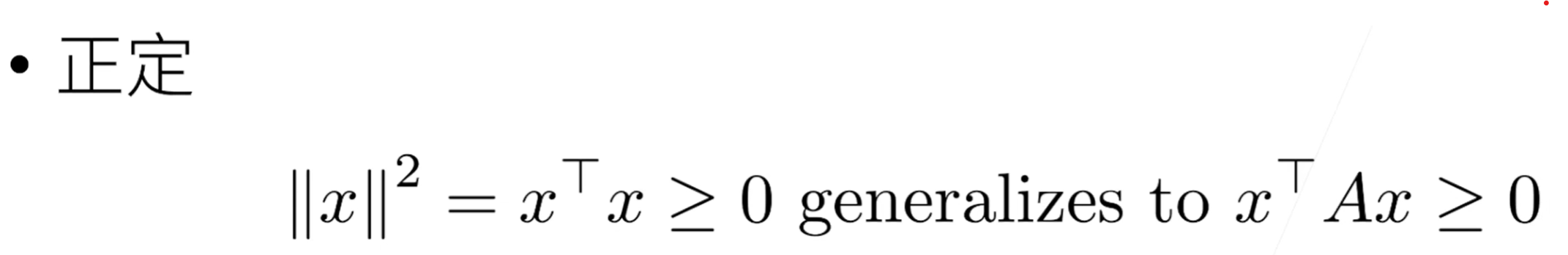
正定矩阵

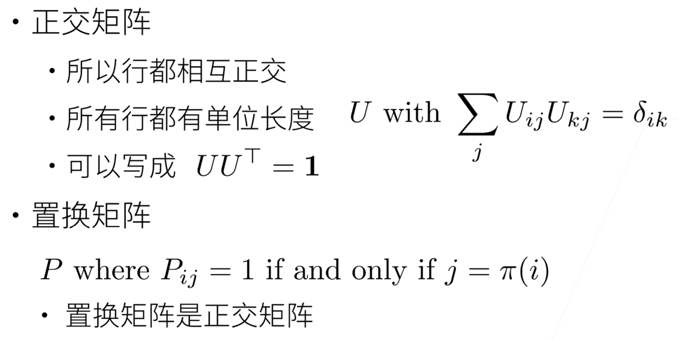
正交矩阵与置换矩阵

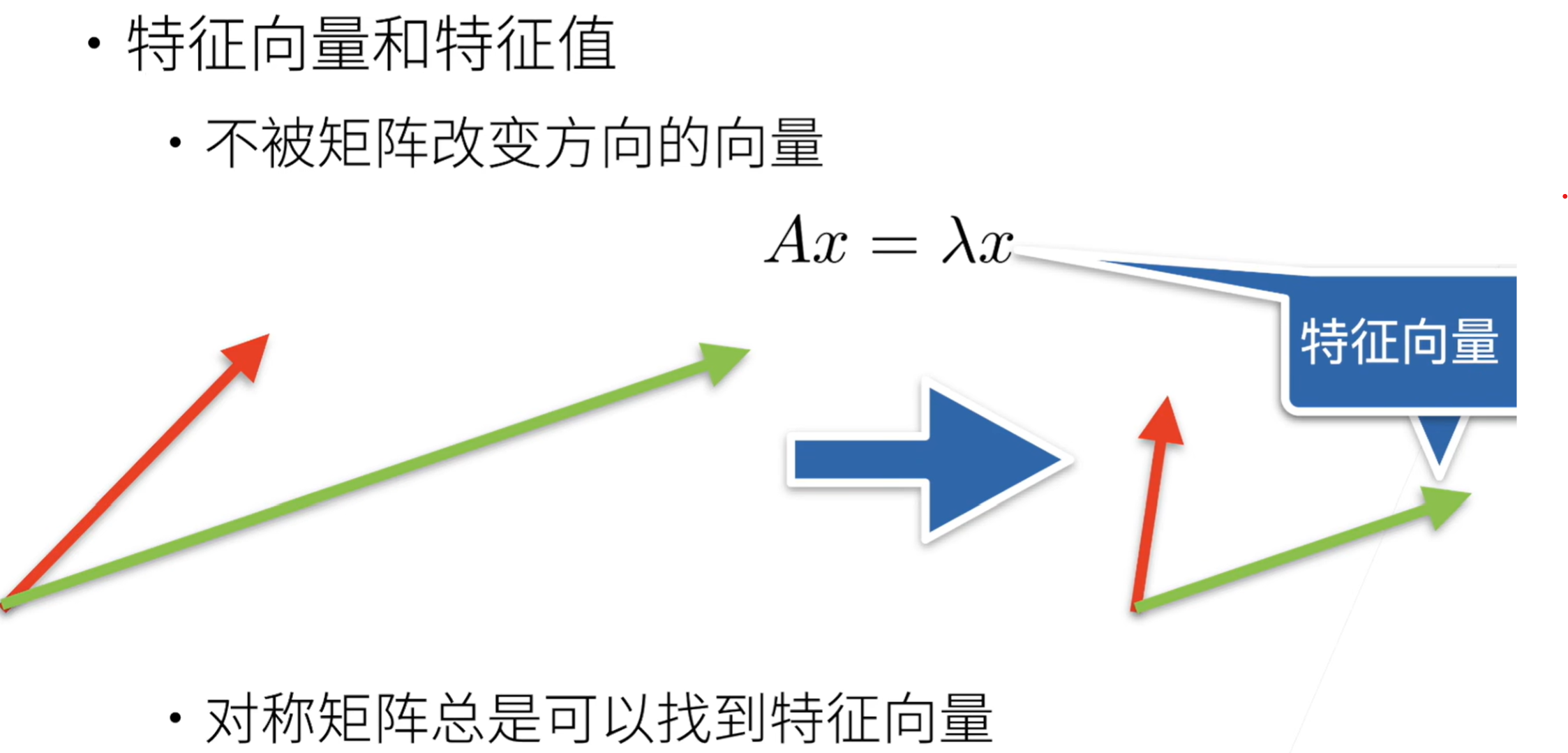
特征向量与特征值

矩阵基本操作

  
import torch

A = torch.arange(20).reshape(5, 4)
A.T # 转置
'''
tensor([[ 0,  4,  8, 12, 16],
        [ 1,  5,  9, 13, 17],
        [ 2,  6, 10, 14, 18],
        [ 3,  7, 11, 15, 19]])
'''

# 对称矩阵
B = torch.tensor([[1, 2, 3], [2, 0, 4], [3, 4, 5]])
B == B.T
'''
tensor([[True, True, True],
        [True, True, True],
        [True, True, True]])
'''

A = torch.arange(20, dtype = torch.float32).reshape(5, 4)
B = A.clone() # 通过分配新内存，将 A 的一个副本分配给 B

# 矩阵按元素相乘 哈达玛积
A * B
'''
tensor([[  0.,   1.,   4.,   9.],
        [ 16.,  25.,  36.,  49.],
        [ 64.,  81., 100., 121.],
        [144., 169., 196., 225.],
        [256., 289., 324., 361.]])
'''

求值

  
'''
(tensor([[ 0.,  1.,  2.,  3.],
         [ 4.,  5.,  6.,  7.],
         [ 8.,  9., 10., 11.],
         [12., 13., 14., 15.],
         [16., 17., 18., 19.]]))
'''

A.sum(axis=0), A.sum(axis=1) # 按行求和 按列求和
'''
(tensor([40., 45., 50., 55.]), tensor([ 6., 22., 38., 54., 70.]))
'''

# 平均值
A.mean(), A.sum() / A.numel()

# 列均值
A.mean(axis=0), A.sum(axis=0) / A.shape[0]

# 计算总和或均值时保持轴数不变
A.sum(axis=1, keepdims=True), A.sum(axis=1, keepdims=False) 
'''
(tensor([[ 6.],
         [22.],
         [38.],
         [54.],
         [70.]]),
 tensor([ 6., 22., 38., 54., 70.]))
'''

# 某个轴计算 A 元素的累积总和
A.cumsum(axis=0), A.cumsum(axis=1)
'''
tensor([[ 0.,  1.,  2.,  3.],
        [ 4.,  6.,  8., 10.],
        [12., 15., 18., 21.],
        [24., 28., 32., 36.],
        [40., 45., 50., 55.]])

tensor([[ 0.,  1.,  3.,  6.],
        [ 4.,  9., 15., 22.],
        [ 8., 17., 27., 38.],
        [12., 25., 39., 54.],
        [16., 33., 51., 70.]])
'''

矩阵各种乘法

  
x = torch.arange(4, dtype=torch.float32)
y = torch.ones(4, dtype=torch.float32)
x, y, torch.dot(x, y) # 点积是相同位置的按元素乘积的和
'''
(tensor([0., 1., 2., 3.]), tensor([1., 1., 1., 1.]), tensor(6.))
'''

# 矩阵向量积
A, x, A.shape, x.shape, torch.mv(A, x) 
'''
(tensor([[ 0.,  1.,  2.,  3.],
         [ 4.,  5.,  6.,  7.],
         [ 8.,  9., 10., 11.],
         [12., 13., 14., 15.],
         [16., 17., 18., 19.]]),
 tensor([0., 1., 2., 3.]),
 torch.Size([5, 4]),
 torch.Size([4]),
 tensor([ 14.,  38.,  62.,  86., 110.]))
'''

# 矩阵 - 矩阵乘法
B = torch.ones(4, 3)
torch.mm(A, B)
'''
tensor([[ 6.,  6.,  6.],
        [22., 22., 22.],
        [38., 38., 38.],
        [54., 54., 54.],
        [70., 70., 70.]])
'''

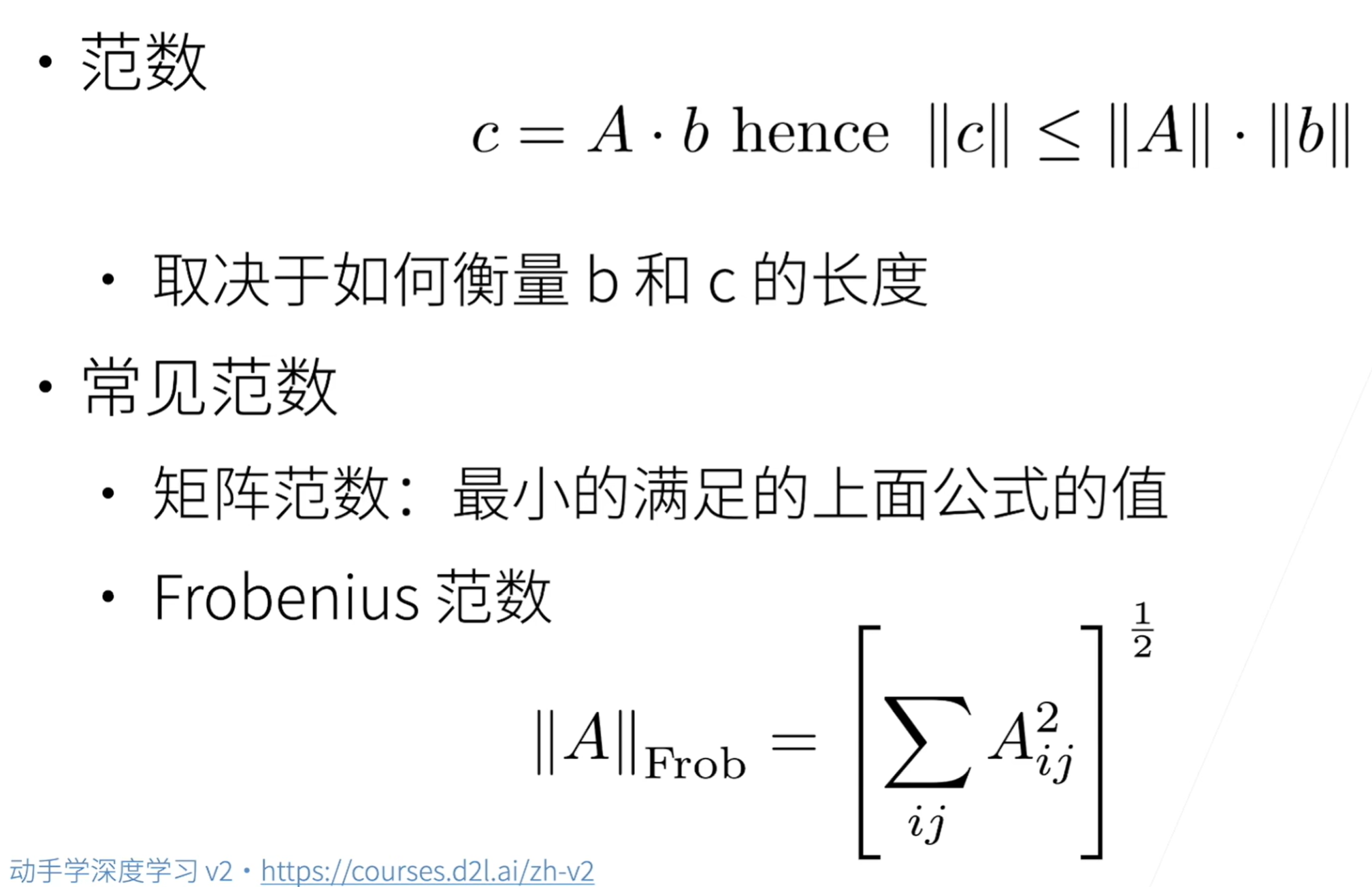
范数

  
# L2 范数是向量元素平方和的平方根
# L1 范数是向量元素的绝对值之和
u = torch.tensor([3,0, -4.0])
torch.norm(u, p=2), torch.abs(u).sum(), torch.norm(u, p=1)
'''
(tensor(5.), tensor(7.), tensor(7.))
'''

# Frobenius 范数是矩阵元素平方和的平方根
torch.norm(torch.ones((4, 9)))
'''
tensor(6.)
'''

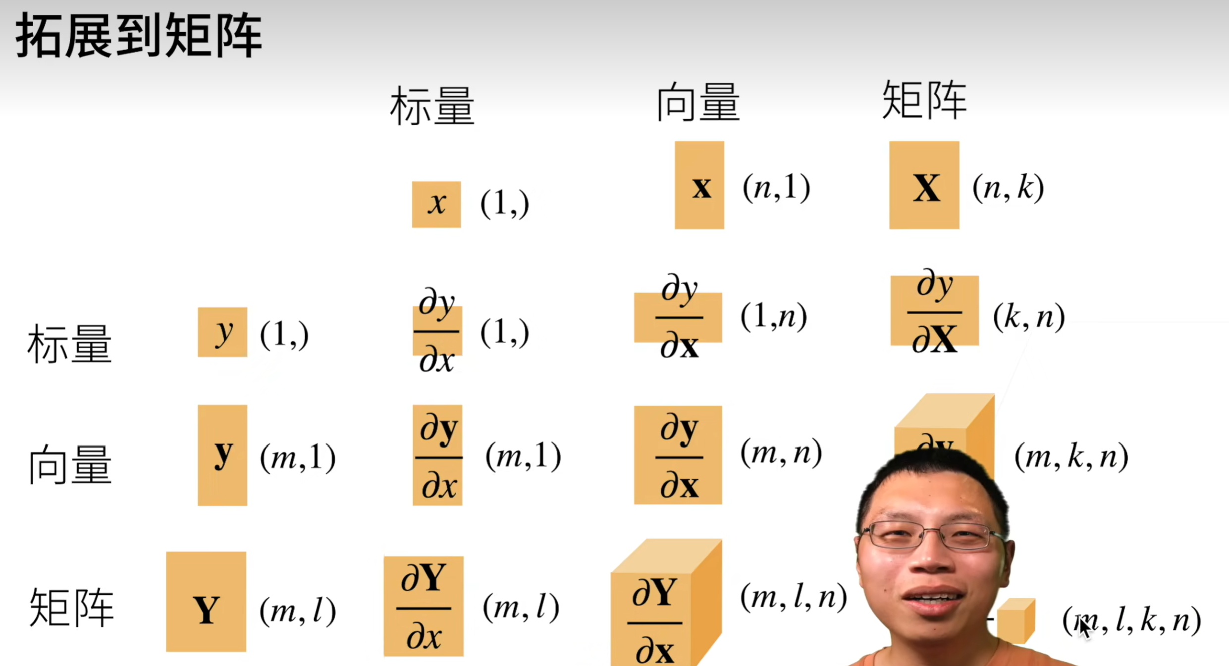
06 矩阵计算

纯数学无代码

07 自动求导

.requires_grad_(True) 允许存储梯度
.backward() 进行反向传播
.grad.zero_() 进行梯度清零，Pytorch 会累积梯度，不会自动清除

  
import torch
x = torch.arange(4.0)
x
'''
tensor([0., 1., 2., 3.])
'''

x.requires_grad_(True)
x.grad # 存储了梯度 默认值是 None

# 等价于 x = torch.arange(4.0, requires_grad=True)

y = 2 * torch.dot(x, x)
y
'''
tensor(28., grad_fn=<MulBackward0>)
'''

# 可以反向传播
y.backward()
x.grad
'''
tensor([ 0.,  4.,  8., 12.])
'''

x.grad == 4 * x
'''
tensor([True, True, True, True])
'''

# 现在让我们计算 x 的另一个函数
# 在默认情况下 pytorch 会累积梯度 所以我们要清楚之前的值
x.grad.zero_()
y = x.sum()
y.backward()
x.grad
'''
tensor([1., 1., 1., 1.])
'''

# 深度学习中 我们的目的不是计算微分矩阵 而是批量中每个样本单独计算的偏导数之和
x.grad.zero_()
y = x * x
# 等价于 y.backward(torch.ones(len(x)))
y.sum().backward()
x.grad
'''
tensor([0., 2., 4., 6.])
'''

# 将某些计算移动到记录的计算图之外
x.grad.zero_()
y = x * x
u = y.detach() # 将 y 从计算图中分离出来
u # u 成了一个常量
'''
tensor([0., 1., 4., 9.])
'''

z = u * x
z.sum().backward()
x.grad == u
'''
tensor([True, True, True, True])
'''

x.grad.zero_()
y = x * x
y.sum().backward()
x.grad == 2 * x
'''
tensor([True, True, True, True])
'''

# 即使构建函数的计算图需要通过 Python 控制流
# 我们仍然可以计算得到的变量的梯度
def f(a):
    b = a * 2
    while b.norm() < 1000:
        b = b * 2
    if b.sum() > 0:
        c = b
    else:
        c = 100 * b
    return c

a = torch.randn(size=(), requires_grad=True)
d = f(a)
d.backward()
a.grad == d / a
'''
tensor(True)
'''

deep learning, limu

deep learning

This post is licensed under CC BY 4.0 by the author.

01 - 03 忽略

04 数据操作 + 数据预处理

基本

计算与连接

内存操作

转换

数据预处理

特别注意 尽量不要改东西

05 线性代数

Frobenius 范数

正定矩阵

正交矩阵与置换矩阵

特征向量与特征值

矩阵基本操作

求值

矩阵各种乘法

范数

06 矩阵计算

纯数学 无代码

07 自动求导

Trending Tags

特别注意尽量不要改东西

纯数学无代码